August 2001
This paper reports a Monte Carlo model of energy transport between particles within a system of one or more reservoirs. It proposes a model based on the hypothesis that energy is transported between particles by means of photon transport. Each particle in the model is assigned a quantum number for the energy contained within a potential well. The model assumes that the energy in each particle's potential well decays periodically, emitting a photon. The model has been implemented using Digital Visual FORTRAN. Using a radiated fraction equal to one third, the calculated density of states within the model fits the Planck radiation equation extremely well. Calculations have been carried out for equilibration, variation of the number of time steps, variation in initial energy, radiation, energy absorption and conduction. A multi-layer model has been used to simulate a temperature gradient.
This paper reports a Monte Carlo model of energy transport between particles within a system of one or more reservoirs. We have previously[1] proposed that photons act in a manner consistent with their possessing negative mass. This has led to the proposition that they might form the means of energy transport between particles with positive mass that have a potential well capable of absorbing them.
The paper proposes a model that uses the above mechanism and makes predictions conforming to the normal observations of physics. That is to say, it is hypothesised that energy is transported between particles by means of photon transport, but in such a way that the model will predict the normally accepted distributions of temperature and energy.
Materials are modelled as one or more contiguous reservoirs. Each reservoir contains a given number of particles, with each particle assigned a quantum number for the energy contained within a potential well. The model assumes that the energy in each particle's potential well decays periodically, emitting a photon. The photon has some probability of leaving the reservoir otherwise it is absorbed by another (possibly the same) particle within the reservoir. If it leaves the reservoir, it will be absorbed by a particle in an adjacent reservoir or, if there is no adjacent reservoir in that direction (i.e. it represents a surface layer), it will be emitted as radiation.
The model assumes that the photon emitted by a particle carries away with it a given fraction of the quantum energy contained within the particle's potential well. The fraction used for any model simulation can be changed so that different possibilities can be studied. If the photon is absorbed by another particle, its energy quantum is added to that of the target particle's potential well. All particles are treated equally and no account is taken of any energy transport as a result of particle movement. This implies that there is no modelling of either convection or transmission via vibration.
The first reservoir in the model can be supplied with mono-energetic photons. This supply represents an external source of energy, such as monochromatic radiation or heating from an electrical source. In the latter case, the photons would rarely be mono-energetic, but the operation of the model is such that there is unlikely to be any time-averaged difference between a stream of mono-energetic photons and a distribution of energies about a mean.
The structure of the model represents a solid body containing one or more layers (the reservoirs). Each layer contains a discrete number of particles and is capable of being at a different temperature to its neighbours. The number of particles in a layer is related to the heat capacity, either via its mass or its specific heat capacity. The implication is that the greater the specific heat capacity, the more particles will interact with the photons for a given mass. The layers have a probability of transmitting photons to their immediate neighbours, representing heat flow between layers.
The emission and absorption of photons within a layer represents the thermal equilibration process, while the transmission of photons to neighbouring layers represents conduction. The emission of photons from the final layer represents radiation from the surface. Both the input photon stream and the transmission between layers can be varied with time allowing, for example, each layer to reach an equilibrium distribution before examining heat flow processes.
The model has been implemented using Digital Visual FORTRAN. Each simulation begins by defining the number of particles in each reservoir and assigning all the particles in each reservoir with a uniform energy quantum number representing the quantum energy within its potential well. For the purpose of the simulation, the energy quantum number is constrained to the range 1 to 231. Each program cycle consists of splitting the energy quantum number of each particle. The fraction split off from the particle is carried away by a photon. The fate of the photon is decided by carrying out Monte Carlo calculations to determine:
Whenever a photon targets a particle, its energy quantum number is added to that of the target particle. Photons that escape are recorded in a transition array for adding to the next layer at the end of the program cycle. Alternatively, photons radiated from the surface layer are assigned to a separate array, which is equivalent to incrementing an integrated detector output. The photons recorded in transition arrays are targeted on particles within the relevant reservoir.
A variable, NSPLIT, controls the fraction of the energy quantum number of each particle that is carried away by each photon it emits. The calculations are entirely in integer arithmetic, so it is impossible to split the energy of a ground state particle with energy quantum number 1. A value of NSPLIT of 2 causes the photon to carry of half of the particle's quantum energy. If NSPLIT has a value of 3, one third is carried off, if it is 4, one quarter, etc.
For the purpose of energy splitting, the quantum number of each particle is recorded prior to the start of the photon propagation calculations. This ensures that the energy fraction carried away by the photon is related to the quantum state at the beginning of the cycle and is not modified by photons targeting the particle during the current program cycle. If the split fraction reflected the modification of a particle's energy quantum number during the cycle, the calculation would become dependent on the order of selection of the particles. Freezing the energy quantum numbers at the beginning of the program cycle avoids the need for an additional Monte Carlo calculation to determine the order of selection for the propagation process.
The output from the simulation is an integrated calculation of the density of states, with individual energies grouped into fifty quantum number bands. The bands are of equal width, ranging from zero to the highest calculated energy. The density of states represents the average number of particles per energy quantum number within each band. For radiation, it represents the average number of photons per energy quantum number within each band radiated since the previous count.
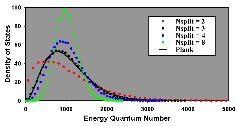
Calculations were performed using a single reservoir with no photon input and no radiation (i.e. a perfectly insulated body). The reservoir contained 216 particles to ensure a good statistical spread. In each case the initial energy quantum number of the particles was 1024. Each simulation comprised 500 program cycles. Trial calculations were performed to ensure that 500 cycles was sufficient to establish equilibrium (see the next section). Calculations were performed using values of NSPLIT equal to 2, 3, 4 and 8. The results are plotted as density of states versus energy quantum number in Figure 1.
Also plotted is the Planck radiation equation:
This has been normalised to a number density by dividing by 4(kT)3/h2c3 and plotting against hf/kT in the normal manner. The Planck equation has been scaled with linear factors for both amplitude and energy quantum number to fit the data. With NSPLIT equal to 3 the fit to the Planck radiation equation is extremely good, given that there will be some statistical variation in the calculated density of states. Based on the results of these calculations and the fit to the Planck radiation equation, all subsequent calculations have been performed using the value of NSPLIT = 3.
Time dependent calculations were performed to ensure that the steady state equilibrium distribution was stable over differing time intervals. Like the previous calculations, the simulation represents a perfectly insulated body. Once again, the reservoir contained 216 particles to ensure a good statistical spread and the initial energy quantum number of the particles was 1024. Results were recorded for a single simulation after 10, 100 and 1000 program cycles. The results are plotted in Figure 2.
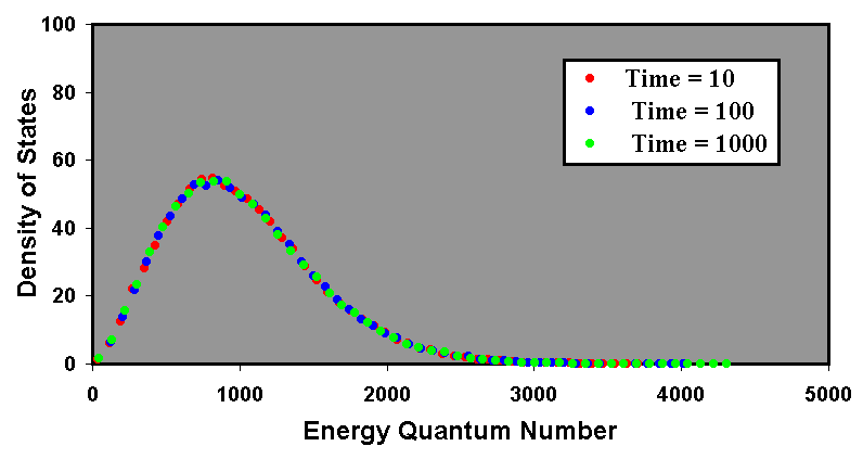
The results indicate that, for a steady state calculation, the simulation reaches equilibrium in less than 10 program cycles. All subsequent calculations use between 64 and 512 program cycles to establish energy quantum equilibrium prior to the investigation of any further phenomena.
Calculations were performed with different values of initial energy quantum number. As with the previous calculations, the simulation represents a perfectly insulated body and the reservoir contained 216 particles to ensure a good statistical spread. Three cases were investigated, with initial energy quantum numbers of 512, 1024 and 2048. Each calculation occupied 100 program cycles. The results are plotted in Figure 3.
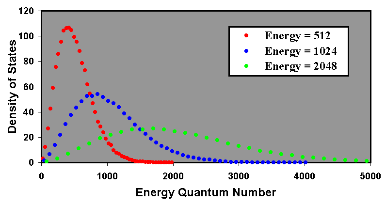
As expected, the peak in the density of states shifts to a higher quantum number as the initial (and therefore mean) energy quantum number increases. Also, the spread of energies increases such that the peak amplitude is inversely proportional to the mean quantum number.
Calculations were performed to consider the effects of black body radiation. As with the previous calculations, and the reservoir contained 216 particles to ensure a good statistical spread. The initial mean energy quantum number was 2048. In this case the simulation began with a perfectly insulated body to establish equilibrium. Thereafter, photons were allowed to radiate from one surface with a probability of 0.01 per emission. Results were generated after 100, 200, 300 and 400 program cycles.
If the split energy at every emission is 1/3 of the reservoir energy of each particle, a fraction of 0.01 for radiation events can be expected to cause a mean energy quantum number loss of 0.0033 of the total. Thus the fraction of the mean energy quantum number retained at the end of a program cycle would be 99.67%. After 200 program cycles (i.e. 100 program cycles of radiation) the residual mean energy quantum number can be expected to be modified by (1 - 0.0033)100, which represents a fall to 71.6% of the original level. After two further periods of 100 program cycles the fraction can be expected to fall to 51.3% and 36.7% respectively. The results are shown in Figure 4.
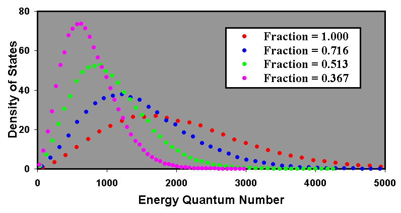
The peak energy quantum number for the four plots is 1701, 1216, 903 and 630. Based on an initial peak position of 1701, the expected peak positions of the other plots, given the calculated decay rates, are respectively 1222, 875 and 626. The peak amplitudes of the density of states are 27, 37.7, 52.6 and 73.6. Based on an initial peak amplitude of 27, the expected peak amplitudes of the other plots, given the calculated decay rates, are respectively 37.7, 52.5 and 73.6. Allowing for the granular nature of the energy quantum number bins, it can be considered that the correlation between the radiation process and the expected fall in temperature is exact.
Calculations were performed to consider the effects of energy absorption. As with the previous calculations, and the reservoir contained 216 particles to ensure a good statistical spread. The initial mean energy quantum number was 512. Once again the simulation begins with a perfectly insulated body to establish equilibrium. Thereafter, source photons were absorbed by the reservoir at the rate of 1024 per program cycle, each have an energy quantum number of 512. Results were generated after 64, 128, 192 and 256 program cycles.
With 1024 source photons per cycle, each with an energy quantum number of 512, the mean energy quantum number within the reservoir at the end of a 64 program cycles of absorption would be 1024, or twice the starting value. This would occur 128 program cycles after the beginning of the simulation. After two further periods of 64 program cycles the mean can be expected to rise to 3 and 4 times the original number. The results are shown in Figure 5.
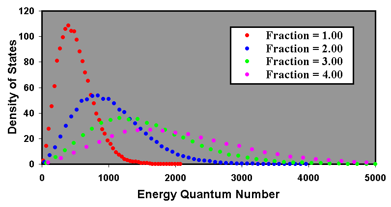
The peak energy quantum number for the four plots is 399, 840, 1165 and 1624. Based on an initial peak position of 399, the expected peak positions of the other plots, given the calculated decay rates, are respectively 798, 1197 and 1596. The peak amplitudes of the density of states are 108, 53.7, 36.1 and 26.7. Based on an initial peak amplitude of 108, the expected peak amplitudes of the other plots, given the calculated decay rates, are respectively 54, 36 and 27. Again allowing for the granular nature of the energy quantum number bins, it can be considered that the correlation between the absorption process and the expected rise in temperature is exact.
Calculations were performed to consider the combined effects of radiation and energy absorption. As with the previous calculations, and the reservoir contained 216 particles to ensure good statistical spread. The initial mean energy quantum number was 512. As usual, the simulation begins with a perfectly insulated body to establish equilibrium. Thereafter, source photons were absorbed by the reservoir at the rate of 1024 per program cycle, each having an energy quantum number of 512. Simultaneously, radiation was simulated from one surface with loss fractions of 0.015, 0.03 and 0.06 per emission. Equilibrium was maintained for 128 program cycles and the results were generated after 2048 program cycles.
With 1024 source photons per cycle, each with an energy quantum number of 512, the mean energy quantum number gain within the reservoir per program cycle of absorption would be 210 × 29 ÷ 216 = 23. If the split energy at every emission is 1/3 of the reservoir energy of each particle, a fraction of 0.015 for radiation events can be expected to cause a mean energy quantum number loss of 0.005 of the total. Thus the mean energy quantum number lost during each program cycle would be 0.005x, where x is the mean energy quantum number of the particles in the reservoir. This leads to the equilibrium equation:
So x = 1600. Where the fraction is 0.03 for radiation events, x = 800 and where the fraction is 0.06, x = 400. The calculated results for these three fractions are shown in Figure 6.
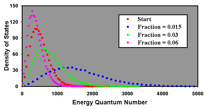
The peak energy quantum number for the four plots is 400, 1426, 637 and 298. Based on an initial peak position of 400, the expected peak positions of the other plots, given the calculated equilibrium factor, are respectively 1250, 625 and 313. The peak amplitudes of the density of states are 107, 35.2, 70.0 and 140. Based on an initial peak amplitude of 107, the expected peak amplitudes of the other plots, given the calculated equilibrium factor, are respectively 34.2, 68.4 and 137. Again allowing for the granular nature of the energy quantum number bins, it can be considered that the correlation between the equilibrium process and the change in temperature is exact.
The calculation with a radiated fraction of 0.015 was used to compare the density of states of the radiated photons with that of the reservoir particles. In this case the number, n, of radiated photons per reservoir particle in 128 time steps is given by:
The results for this calculation are shown in Figure 7.
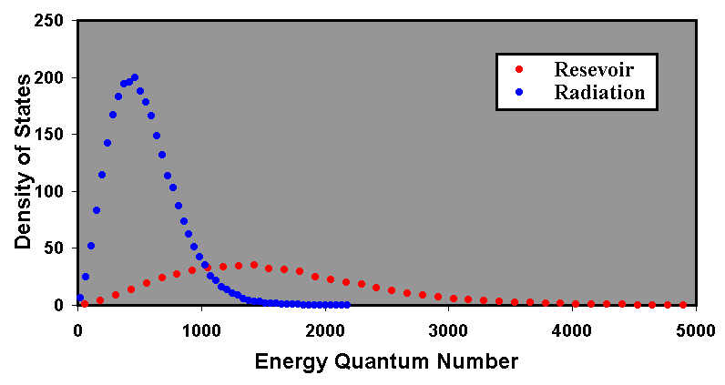
The peak energy quantum numbers for the reservoir and the radiation are 1426 and 462 respectively. The peak densities of state for the two peaks are respectively 35.2 and 200. Because the photons carry off one third of the particle energy when emitted, it can be expected that the energy quantum number for the peak of for the radiation will be one third that of the reservoir particles. The calculated value is quite close to the expected value of 475. With a quantum number of one third that of the reservoir particles, the density of states of the peak for the radiation can be expected to be three times that for the reservoir particles. Multiplying by the peak amplitude for the reservoir particles by 3 × 1.92 (from 3 above) gives an expected peak value for the radiation of 203, which is a good match for the calculated value.
Conduction through layers has been simulated using the multi-reservoir model described earlier. During the conduction process, the model represents a cuboid that has been perfectly insulated on five sides, with net heat flow in a single dimension. In this case, photons leave the first reservoir through one boundary only, whereas for subsequent layers, there are two possible boundaries for exit. To make the radiation calculations consistent with those reported in the previous sections, the probability of a photon escaping from a reservoir, other than the first, must be twice that used in the single reservoir calculations (see below). Hence, if the probability of escape from the single reservoir was 0.06, the probability of escape from the multi-reservoir model must be 0.12, to give 0.06 from each surface.
To ensure that results from simulations with differing numbers of layers are comparable, it is essential to model the fraction of escaping photons consistently. Consider a particle, P, a distance x from the boundary surface B1 of a reservoir where the mean free path is L. Figure 8 represents a cross section of such a reservoir, where it is assumed that the reservoir is infinite in the directions parallel to the boundary surfaces and the two boundaries are denoted by B1 and B2. The angular lines represent the boundary of a cone, within which the distance from P to B1 will be less than L.
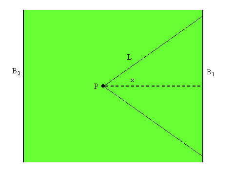
It can be shown that the probability that a photon radiated from P will be along a path contained within the cone is ½(1 - x/L). If it is assumed that the distribution of photon path lengths is normal about the mean, then the probability that photon will escape through the boundary can be reduced to whether or not its path length to the boundary is less than the mean free path. If the thickness, T, of the reservoir is exactly L, the probability, Pr (B1), that any photon will be radiated through B1 is given by:
This gives Pr (B1) as 0.25. For T greater than L the integral becomes
For T less than L it becomes
So for T = 2L we have Pr(B1) = 0.125 and for T = 4L, Pr(B1) = 0.0625, etc. In other words, for T > L (i.e. Pr(B1) < 0.25), Pr(B1) ∝ L/T. For T = L/2 we have Pr(B1) = 0.375 and for T = L/4, Pr(B1) = 0.4375, etc. In other words, for T < L (i.e. Pr(B1) > 0.25), the probability, ½-Pr(B1), that the photon will not pass through boundary B1 is given by ½-Pr(B1), ∝ L/T.
So far we have considered only the single boundary B1. However, except in the case of the first reservoir, which we assume to be perfectly insulated at one end, there is a second boundary, B2, which must be considered. The overall probability that a photon will not pass through either boundary is
In the case of T»L, the overall probability of transmission is approximately 2Pr (B1).
The change from single reservoir to multi-reservoir model has two interpretations. One is that two or more pieces of material, each identical to that of the single reservoir model, are fused together along the axis of net heat flow. The other is that the single reservoir is considered from the viewpoint of a smaller scale length. In the first case, the probability of transmission must be kept the same as for the single reservoir model. The mean energy quantum number input per particle in the first reservoir is equivalent to the same energy input as in the single reservoir model. In the second case, the probability of transmission must be increased to reflect the decrease in layer thickness, as described above. The mean energy quantum number input per particle in the first reservoir must be increased to remain equivalent to the same energy input as in the single reservoir model.
For a single reservoir with a mean energy quantum number input of 8 per particle and a value of Pr (B1) of 0.03 the equilibrium mean energy quantum number, a, for the reservoir will be given by:
The value of 0.01 comes from the energy split function (0.03/3). Thus a = 800. Now consider a 2-reservoir model of the fused reservoir type. With the same equilibrium conditions, and where b is the equilibrium mean energy quantum number for Reservoir 2, we have:
This gives a = 1600 and b = 800. In other words the surface temperature (Reservoir 2 mean energy quantum number) is the same as that of the single reservoir model for the same energy radiation loss. However, the internal temperature gradient, which drives the heat transfer process, leads to a higher core temperature (Reservoir 1 mean energy quantum number). If we reduce T/L by a factor of 2 so that Pr (B1) = 0.06, we would require a mean energy quantum number input of 16 per particle to maintain the same equilibrium conditions. This is described by the equations:
Once again, a = 1600 and b = 800. So although the two types model different physical systems, the results are the same, which is not unexpected, given the relationship between them.
A calculation was performed for a model with 5 reservoirs. Each reservoir had 216 particles, each with an initial energy quantum number of 512 and there were 512 program cycles for equilibration. There were 1024 input photons per times step, each with an energy quantum number of 512. Thus the mean energy quantum number input was 8 per particle. The simulation was performed with a probability of escape of 0.03 through a single interface and 0.06 through two interfaces. The value of 0.06 is slightly higher than the exact value obtained via equation 7 of 0.0591, but has been used for simple comparison with deterministic calculations. The results of the simulation are shown in Figure 9.
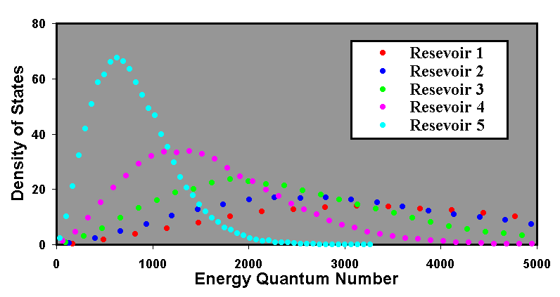
The results represent the output after 213 program cycles. Equilibrium was reached after about 3 x 211 program cycles. The mean energies can be calculated deterministically via a set of parametric equations:
The values of a, b, c, d and e are the mean energy quantum numbers of the five reservoirs. The equations predict values of a = 4000, b = 3200, c = 2400, d = 1600 and e = 800. The actual values calculated by the simulation were respectively 3981, 3204, 2390, 1602 and 801.
A model has been proposed to account for the conduction process by assuming energy transport via photon emission and absorption. A value of 1/3 has been assigned to the fraction of the energy quantum number within a particle's potential well that is radiated when a photon is emitted. The simulation output fits the Planck radiation equation very well. The model can be used to model the conduction process by modelling material as a finite number of discrete layers. The results are in good agreement with the predictions of classical thermodynamics.
[1] L D Howe Symmetry Between Gravitational and Electric Forces, www.innovationgame.com/physics (2000).